Physics TORQUE ON CURRENT LOOP, MAGNETIC DIPOLE , CIRCULAR CURRENT AS A MAGNETIC DIPOLE, THE MOVING COIL GALVANOMETER FOR CBSE-NCERT 4

Topic covered

`color{blue}{star}` TORQUE ON CURRENT LOOP, MAGNETIC DIPOLE
`color{blue}{star}` CIRCULAR CURRENT AS A MAGNETIC DIPOLE
`color{blue}{star}` THE MOVING COIL GALVANOMETER

Torque on a rectangular current loop in a uniform magnetic field

`color{blue} ✍️` We now show that a rectangular loop carrying a steady current `I` and placed in a uniform magnetic field experiences a torque.

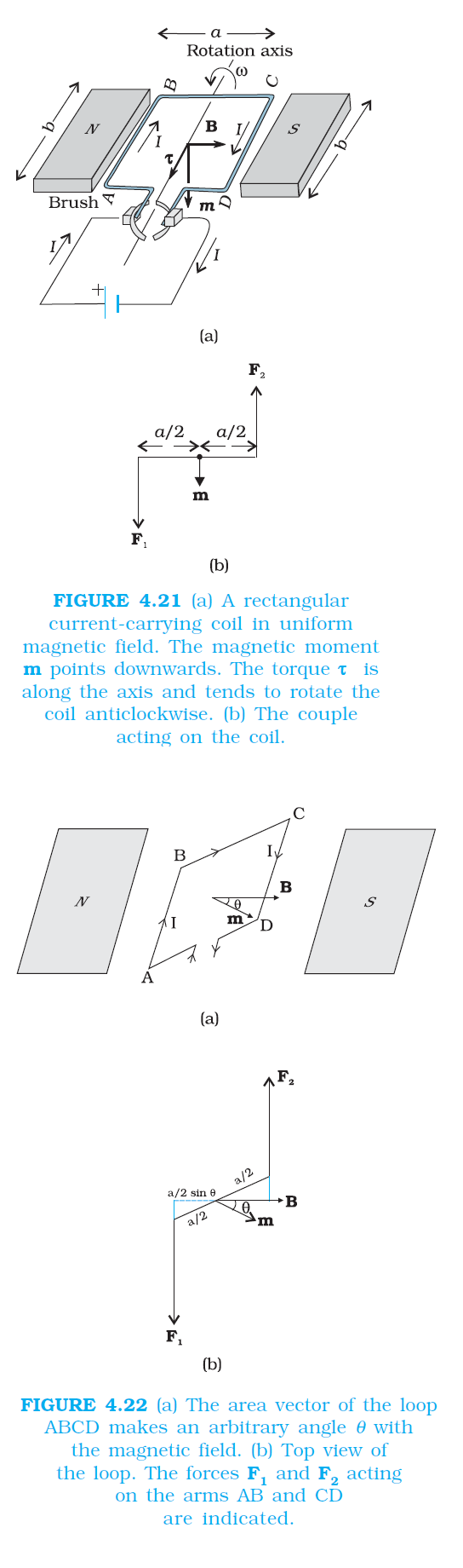
`color {blue}{➢➢}`It does not experience a net force. This behaviour is analogous to that of electric dipole in a uniform electric field (Section 1.10). We first consider the simple case when the rectangular loop is placed such that the uniform magnetic field `B` is in the plane of the loop.

`color {blue}{➢➢}`This is illustrated in Fig. 4.21(a). The field exerts no force on the two arms `AD` and `BC` of the loop. It is perpendicular to the arm `AB` of the loop and exerts a force `F_1` on it which is directed into the plane of the loop. Its magnitude is,

`color{blue}(F_1 = IbB)`

`color {blue}{➢➢}`Similarly it exerts a force `F_2` on the arm `CD` and `F_2` is directed out of the plane of the paper.

`color{blue}(F_2 = I b B = F_1)`

`color {blue}{➢➢}`Thus, the net force on the loop is zero. There is a torque on the loop due to the pair of forces `F_1` and `F_2.` Figure 4.21(b) shows a view of the loop from the `AD` end. It shows that the torque on the loop tends to rotate it anti-clockwise. This torque is (in magnitude).

`color{blue}(tau = F_1 a/2 + F_2a/2)`

`color{blue}(= IbB a/2 + I bB a/2 = I(ab)B)`

` color{blue}(= IAB)`

..........(4.26)

`color {blue}{➢➢}`where `A = ab` is the area of the rectangle.

We next consider the case when the plane of the loop, is not along the magnetic field, but makes an angle with it. We take the angle between the field and the normal to the coil to be angle `θ` (The previous case
corresponds to `θ = π/2`).

`color{blue} ✍️` Figure 4.22 illustrates this general case. The forces on the arms `BC` and `DA` are equal, opposite, and act along the axis of the coil, which connects the centres of mass of `BC` and `DA`.


`color {blue}{➢➢}` Being collinear along the axis they cancel each other, resulting in no net force or torque. The forces on arms `AB` and `CD` are `F_1` and `F_2`. They too are equal and opposite, with magnitude, `F_1 = F_2 = I bB` But they are not collinear! This results in a couple as before.

`color{blue} ✍️` The torque is, however, less than the earlier case when plane of loop was along the magnetic field. This is because the perpendicular distance between the forces of the couple has decreased. Figure 4.22(b) is a view of the arrangement from the AD end and it illustrates these two forces constituting a couple. The magnitude of the torque on the loop is,

`color{blue}(tau = F_1 a/2 sin theta + F_2 a/2 sin theta)`
`color{blue}(=I ab B sin θ)`

`color{blue}(= I A B sin θ)`

.........(4.27)

`color {blue}{➢➢}` As `color{blue}(θ -> 0,)` the perpendicular distance between the forces of the couple also approaches zero. This makes the forces collinear and the net force and torque zero.

`color{blue} ✍️`The torques in Eqs. (4.26) and (4.27) can be expressed as vector product of the magnetic moment of the coil and the magnetic field. We define the magnetic moment of the current loop as,

`color{blue}{m = I A}`

..............(4.28)

`color {blue}{➢➢}` where the direction of the area vector `A` is given by the right-hand thumb rule and is directed into the plane of the paper in Fig. 4.21. Then as the angle between `m` and B is `θ` , Eqs. (4.26) and (4.27) can be expressed by one expression

`color{blue}{τ = m × B}`

............(4.29)

`color{blue} ✍️` This is analogous to the electrostatic case (Electric dipole of dipole moment `p_e` in an electric field `E`).

`color{blue}(tau = P_e xx E)`

`color {blue}{➢➢}` As is clear from Eq. (4.28), the dimensions of the magnetic moment are `[A][L^2]` and its unit is `Am^2.` From Eq. (4.29), we see that the torque `τ` vanishes when `m` is either parallel or antiparallel to the magnetic field `B`.

`color {blue}{➢➢}` This indicates a state of equilibrium as there is no torque on the coil (this also applies to any object with a magnetic moment `m`). When `m` and `B` are parallel the equilibrium is a stable one. Any small rotation of the coil produces a torque which brings it back to its original position.

`color {blue}{➢➢}` When they are antiparallel, the equilibrium is unstable as any rotation produces a torque which increases with the amount of rotation. The presence of this torque is also the reason why a small magnet or any magnetic dipole aligns itself with the external magnetic field. If the loop has `N` closely wound turns, the expression for torque, Eq. (4.29), still holds, with.

`color{blue}(m = N I A)`

...............(4.30)
Q 3165701665

A 100 turn closely wound circular coil of radius 10 cm carries a current of 3.2 A. (a) What is the field at the centre of the coil? (b) What is The coil is placed in a vertical plane and is free to rotate about a horizontal axis which coincides with its diameter. A uniform magnetic field of `2T` in the horizontal direction exists such that initially the axis of the coil is in the direction of the field. The coil rotates through an angle of `90º` under the influence of the magnetic field. (c) What are the magnitudes of the torques on the coil in the initial and final position? (d) What is the angular speed acquired by the coil when it has rotated by `90º?` The moment of inertia of the coil is `0.1 kg m_2.` the magnetic moment of this coil?
Class 12 Chapter example 11
Solution:

(a) From Eq. (4.16)

`B = (mu_0NI)/(2R)`

Here, `N = 100; I = 3.2 A,` and `R = 0.1 m`. Hence,

`B=(4pixx10^(-7)xx10^2xx3.2)/(2xx10^(-T)) = (4xx10^(-5)xx10)/(2xx10^(-1))`

The direction is given by the right-hand thumb rule.
(b) The magnetic moment is given by Eq. (4.30),
`m = N I A = N I π r^2 = 100 × 3.2 × 3.14 × 10^(–2) = 10 A m^2`

The direction is once again given by the right hand thumb rule.

`(c) τ = m × B` [from Eq. (4.29)]
`= m B sin theta`
Initially, `θ = 0.` Thus, initial torque τ `i = 0`. Finally, `θ = π/2 (or 90º).` Thus, final torque `t_i = m B = 10 × 2 = 20 N m.`

(d) From Newton’s second law,

`g(domega)/(dt) m B sin theta`

where `g` is the moment of inertia of the coil. From chain rule,

`(domega)/(dt) = (domega)/(dtheta) = (domega)/(dtheta)omega`

Using this,

`gω dω = m B sinθ dθ`

Integrating from `θ = 0` to `θ = π/2,`

`g int_(0)^(omega) omega d omega = m B int_(0)^(x//2) sin theta d theta`

`g (omega_(f)^(2))/(2) = -m B cos theta |_(0)^(x//2) = mB`

`omega_f (2mB)/(g)^(1//2) = (2xx20)/(10^(-1))^(1//2) = 20 s^(-1)`
Q 3185701667

(a) A current-carrying circular loop lies on a smooth horizontal plane. Can a uniform magnetic field be set up in such a manner that the loop turns around itself (i.e., turns about the vertical axis).
(b) A current-carrying circular loop is located in a uniform external magnetic field. If the loop is free to turn, what is its orientation of stable equilibrium? Show that in this orientation, the flux of the total field (external field + field produced by the loop) is maximum.
(c) A loop of irregular shape carrying current is located in an external magnetic field. If the wire is flexible, why does it change to a circular shape?
Class 12 Chapter example 12
Solution:

(a) No, because that would require τ to be in the vertical direction. But `τ = I A × B`, and since A of the horizontal loop is in the vertical direction, τ would be in the plane of the loop for any B.
(b) Orientation of stable equilibrium is one where the area vector A of the loop is in the direction of external magnetic field. In this orientation, the magnetic field produced by the loop is in the same direction as external field, both normal to the plane of the loop, thus giving rise to maximum flux of the total field.
(c) It assumes circular shape with its plane normal to the field to maximize flux, since for a given perimeter, a circle encloses greater area than any other shape.

CIRCULAR CURRENT AS A MAGNETIC DIPOLE

`color{blue} ✍️` In this section, we shall consider the elementary magnetic element: the current loop. We shall show that the magnetic field (at large distances) due to current in a circular current loop is very similar in behavior to the electric field of an electric dipole.

`color {blue}{➢➢}` In Section 4.6, we have evaluated the magnetic field on the axis of a circular loop, of a radius `R`, carrying a steady current `I`. The magnitude of this field is [(Eq. (4.15)],

`color{blue}(B = (mu_0IR^2)/(2(x^2 + R^2)^(3//2)))`

`color {blue}{➢➢}` and its direction is along the axis and given by the right-hand thumb rule (Fig. 4.12).

`color {blue}{➢➢}` Here, `x` is the distance along the axis from the centre of the loop. For `x > > R,` we may drop the `R^2` term in the denominator. Thus,

`color{blue}(B = (mu_0R^2)/(2x^3))`

`color {brown}{"Note that"}` the area of the loop `color{blue}(A = πR^2.)` Thus,

`color{blue}(B= (mu_0IA)/(2pix^3))`

`color {blue}{➢➢}` As earlier, we define the magnetic moment `m` to have a magnitude , `color{blue}(m = I A)`. Hence,

`color{blue}(B approx (mu_0M)/(2pix^3))`

`color{blue}(= (mu_0)/(4pi) (2m)/(x^3))`

..............[4.31(a)]

`color {blue}{➢➢}`The expression of Eq. [4.31(a)] is very similar to an expression obtained earlier for the electric field of a dipole. The similarity may be seen if we substitute,

`color{blue}(mu-> 1/epsilon_0)`

`color{blue}(M-P_e ("electrostatic dipole"))`
`color{blue}(B → E ("electrostatic field) We then obtain,")`

`color{blue}(E = (2P_e)/(4piepsilon_0x^3))`

`color {blue}{➢➢}`which is precisely the field for an electric dipole at a point on its axis. considered in Chapter 1, Section 1.10 [Eq. (1.20)].

`color {blue}{➢➢}` It can be shown that the above analogy can be carried further. We had found in Chapter 1 that the electric field on the perpendicular bisector of the dipole is given by [See Eq.(1.21)],

`color{blue}(E ≃ (P_e)/(4piepsilon_0x^3))`

`color {blue}{➢➢}` where `x` is the distance from the dipole. If we replace `p -> m` and `color{blue}(μ_0 →1/ε_0)` in the above expression, we obtain the result for `B` for a point in the plane of the loop at a distance x from the centre. For `x > >R,`

`color{blue}(B ≃ (mu_0)/(4pi) m/(x^3) ; x > > R)`

...............[4.31(b)]

`color {blue}{➢➢}` The results given by Eqs. [4.31(a)] and [4.31(b)] become exact for a point magnetic dipole.

`color {blue}{➢➢}` The results obtained above can be shown to apply to any planar loop: a planar current loop is equivalent to a magnetic dipole of dipole moment `m = I A,` which is the analogue of electric dipole moment `p`.

`color{brown}bbul {"Note}`, however, a fundamental difference: an electric dipole is built up of two elementary units — the charges (or electric monopoles). In magnetism, a magnetic dipole (or a current loop) is the most elementary element.

`color{blue} ✍️` The equivalent of electric charges, i.e., magnetic monopoles, are not known to exist. We have shown that a current loop `color {blue}{(i)}` produces a magnetic field (see Fig. 4.12) and behaves like a magnetic dipole at large distances, and
`color {blue}{(ii)}` is subject to torque like a magnetic needle.

`color {blue}{➢➢}` This led Ampere to suggest that all magnetism is due to circulating currents. This seems to be partly true and no magnetic monopoles have been seen so far. However, elementary particles such as an electron or a proton also carry an intrinsic magnetic moment, not accounted by circulating currents.

The magnetic dipole moment of a revolving electron

`color{blue} ✍️` We shall read about the Bohr model of the hydrogen atom. You may perhaps have heard of this model which was proposed by the Danish physicist Niels Bohr in 1911 and was a stepping stone to a new kind of mechanics, namely, quantum mechanics.

`color {blue}{➢➢}` In the Bohr model, the electron (a negatively charged particle) revolves around a positively charged nucleus much as a planet revolves around the sun. The force in the former case is electrostatic (Coulomb force) while it is gravitational for the planet-Sun case. We show this Bohr picture of the electron in Fig. 4.23.

`color{blue} ✍️` The electron of charge `color{blue}((–e) (e = + 1.6 × 10^(–19) C))` performs uniform circular motion around a stationary heavy nucleus of charge `+Ze`. This constitutes a current `I`, where,

`color{blue}(I = e/T)`

............(4.32)

and `T` is the time period of revolution. Let `r` be the orbital radius of the electron, and `v` the orbital speed.

Then,

`color{blue}(T = (2pir)/(v))`

...............(4.33)

`color {blue}{➢➢}` Substituting in Eq. (4.32), we have `color{blue}(I = (ev)/(2πr).)` There will be a magnetic moment, usually denoted by `μ_l,` associated with this circulating current. From Eq. (4.28) its magnitude is, `color{blue}(μ_l = Iπr^2 = (evr)/2.)`

`color {blue}{➢➢}` The direction of this magnetic moment is into the plane of the paper in Fig. 4.23. [This follows from the right-hand rule discussed earlier and the fact that the negatively charged electron is moving anti-clockwise, leading to a clockwise current.] Multiplying and dividing the right-hand side of the above expression by the electron mass `m_e`, we have,

`color{blue}(mu_l = e/(2m_e)(m_evr))`

`color{blue}(= e/(2m_e)l)`

...........[4.34(a)]

`color {blue}{➢➢}` Here, `l` is the magnitude of the angular momentum of the electron about the central nucleus (“orbital” angular momentum). Vectorially,

`color{blue}(mu_l= - (e)/(2m_e)l)`

............[4.34(b)]

`color {blue}{➢➢}` The negative sign indicates that the angular momentum of the electron is opposite in direction to the magnetic moment. Instead of electron with charge `(–e)`, if we had taken a particle with charge `(+q)`, the angular momentum and magnetic moment would be in the same direction.

`color{blue}((mu_l)/l = e/(2m_e))`

...........(4.35)

`color {blue}{➢➢}` The ratio is called the gyromagnetic ratio and is a constant. Its value is `8.8 × 10^(10) C // kg` for an electron, which has been verified by experiments.

`color{blue} ✍️` The fact that even at an atomic level there is a magnetic moment, confirms Ampere’s bold hypothesis of atomic magnetic moments. This according to Ampere, would help one to explain the magnetic properties of materials. Can one assign a value to this atomic dipole moment? The answer is Yes. One can do so within the Bohr model. Bohr hypothesised that the angular momentum assumes a discrete set of values, namely,

`color{blue}(l = (nh)/(2pi))`

................(4.36)

`color {blue}{➢➢}` where `n` is a natural number, `color{blue}(n = 1, 2, 3, ....)` and `h` is a constant named after Max Planck (Planck’s constant) with a value h `color{blue}(= 6.626 × 10^(–34) J s.)` This condition of discreteness is called the Bohr quantisation condition.

`color{blue} ✍️` We shall discuss it in detail in Chapter 12. Our aim here is merely to use it to calculate the elementary dipole moment. Take the value `n = 1,` we have from Eq. (4.34) that,

`color{blue}((mu_l)_(min) = (e)/(4pim_e)h)`

`color{blue}(= (1.60xx 10^(-19) xx 6.63xx 10^(-34))/(4xx3.14 xx 9.11xx10^(-31)))`

`color{blue}(= 9.27xx 10^(-24) Am^2)`

.................(4.37)

`color {blue}{➢➢}` where the subscript ‘min’ stands for minimum. This value is called the Bohr magneton,

`color {blue}{➢➢}` Any charge in uniform circular motion would have an associated magnetic moment given by an expression similar to Eq. (4.34). This dipole moment is labelled as the orbital magnetic moment. Hence the subscript `l` in `μ_l` .

`color {blue}{➢➢}` Besides the orbital moment, the electron has an intrinsic magnetic moment, which has the same numerical value as given in Eq. (4.37). It is called the spin magnetic moment. But we hasten to add that it is not as though the electron is spinning.

`color {blue}{➢➢}` The electron is an elementary particle and it does not have an axis to spin around like a top or our earth. Nevertheless it does possess this intrinsic magnetic moment. The microscopic roots of magnetism in iron and other materials can be traced back to this intrinsic spin magnetic moment.

THE MOVING COIL GALVANOMETER

`color{blue} ✍️` Currents and voltages in circuits have been discussed extensively in Chapters 3. But how do we measure them? How do we claim that current in a circuit is 1.5 A or the voltage drop across a resistor is `1.2 V`.

`color {blue}{➢➢}` Figure 4.24 exhibits a very useful instrument for this purpose: the moving coil galvanometer (MCG). It is a device whose principle can be understood on the basis of our discussion in Section 4.10.

`color{blue} ✍️` The galvanometer consists of a coil, with many turns, free to rotate about a fixed axis (Fig. 4.24), in a uniform radial magnetic field. There is a cylindrical soft iron core which not only makes the field radial but also increases the strength of the magnetic field.

`color{blue} ✍️` When a current flows through the coil, a torque acts on it. This torque is given by Eq. (4.26) to be

`color{blue}(tau = NIAB)`

`color {blue}{➢➢}` where the symbols have their usual meaning. Since the field is radial by design, we have taken sin `θ = 1` in the above expression for the torque. The magnetic torque `NIAB` tends to rotate the coil. A spring `S_p` provides a counter torque `kphi` that balances the magnetic torque `NIAB;` resulting in a steady angular deflection `phi`. In equilibrium

`color{blue}(kphi = NI AB)`

`color {blue}{➢➢}` where `k` is the torsional constant of the spring; i.e. the restoring torque per unit twist. The deflection `phi` is indicated on the scale by a pointer attached to the spring. We have

`color{blue}(phi = (NAB)/(k)I)`

..................(4.38)

`color {blue}{➢➢}` The quantity in brackets is a constant for a given galvanometer. The galvanometer can be used in a number of ways. It can be used as a detector to check if a current is flowing in the circuit.

`color {blue}{➢➢}` We have come across this usage in the Wheatstone’s bridge arrangement. In this usage the neutral position of the pointer (when no current is flowing through the galvanometer) is in the middle of the scale and not at the left end as shown in Fig.4.24.

`color {blue}{➢➢}` Depending on the direction of the current, the pointer deflection is either to the right or the left. The galvanometer cannot as such be used as an ammeter to measure the value of the current in a given circuit.

`color{blue} ✍️` This is for two reasons:
`color {blue}{(i)}` Galvanometer is a very sensitive device, it gives a full-scale deflection for a current of the order of `μA`.
`color {blue}{(ii)}` For measuring currents, the galvanometer has to be connected in series, and as it has a large resistance, this will change the value of the current in the circuit.

`color{blue} ✍️` To overcome these difficulties, one attaches a small resistance rs, called shunt resistance, in parallel with the galvanometer coil; so that most of the current passes through the shunt. The resistance of this arrangement is,

`color{blue}(R_G r_S//(R_G+r_S) ≃ r_s " " "if" " " R_G > > r_s)`

`color{blue} ✍️` If `r_s` has small value, in relation to the resistance of the rest of the circuit `R_c,` the effect of introducing the measuring instrument is also small and negligible.


`color{blue} ✍️` This arrangement is schematically shown in Fig. 4.25. The scale of this ammeter is calibrated and then graduated to read off the current value with ease. We define the current sensitivity of the galvanometer as the deflection per unit current. From Eq. (4.38) this current sensitivity is,

`color{blue}((phi)/I = (NAB)k)`

.........(4.39)

`color{blue} ✍️` A convenient way for the manufacturer to increase the sensitivity is to increase the number of turns `N`. We choose galvanometers having sensitivities of value, required by our experiment.

`color{blue} ✍️` The galvanometer can also be used as a voltmeter to measure the voltage across a given section of the circuit. For this it must be connected in parallel with that section of the circuit. Further, it must draw a very small current, otherwise the voltage measurement will disturb the original set up by an amount which is very large.


`color{blue} ✍️` Usually we like to keep the disturbance due to the measuring device below one per cent. To ensure this, a large resistance R is connected in series with the galvanometer. This arrangement is schematically depicted in Fig.4.26. Note that the resistance of the voltmeter is now,

`color{blue}(R_G + R ≃ R " " " large")`

`color{blue} ✍️` The scale of the voltmeter is calibrated to read off the voltage value with ease. We define the voltage sensitivity as the deflection per unit voltage. From Eq. (4.38),

`color{blue}((phi)/V = = (NAB)/k I/V= ((NAB)/k) 1/R)`

...............(4.40)

`color{blue} ✍️` An interesting point to note is that increasing the current sensitivity may not necessarily increase the voltage sensitivity. Let us take Eq. (4.39) which provides a measure of current sensitivity. If `color{blue}(N → 2N,)` i.e., we double the number of turns, then

`color{blue}((phi)/I -> 2(phi)/I)`

`color {blue}{➢➢}` Thus, the current sensitivity doubles. However, the resistance of the galvanometer is also likely to double, since it is proportional to the length of the wire. In Eq. (4.40), `color{blue}(N →2N)`, and `color{blue}(R →2R,)` thus the voltage sensitivity,

`color{blue}((phi)/V-> (phi)/V)` remains unchanged. So in general, the modification needed for conversion of a galvanometer to an ammeter will be different from what is needed for converting it into a voltmeter.
Q 3125801761

In the circuit (Fig. 4.27) the current is to be measured. What is the value of the current if the ammeter shown (a) is a galvanometer with a resistance `R_G = 60.00 Ω;` (b) is a galvanometer described in (a) but converted to an ammeter by a shunt resistance `r_s = 0.02 Ω; (c)` is an ideal ammeter with zero resistance?
Class 12 Chapter example 13
Solution:

(a) Total resistance in the circuit is,
`R_G + 3 =63 Ω.` Hence, `I = 3/63 = 0.048 A.`
(b) Resistance of the galvanometer converted to an ammeter is,

`(R_GR_X)/(R_G+r_X) = (60omegaxx0.02Ω)/((60+0.02)Ω`
Total resistance in the circuit is,
`0.02Ω + 3Ω = 3.02Ω .` Hence, `I = 3/3.02 = 0.99 A.`
(c) For the ideal ammeter with zero resistance,
`I = 3/3 = 1.00 A`

 
SiteLock